![]()
🐾 Introduction to object detection and tracking#
This notebook gives a practical introduction to blob detection and particle tracking in the context of a 2D cell lineage tracing challenge.
Note
This notebook was adapted from an example from napari.org which you can check out here: Single cell tracking with napari.
Setup#
First, check that you have all the necessary packages installed, including napari and trackpy.
import napari
import trackpy as tp
Tip
If you are executing this notebook on a Jupyter Hub, launch a Remote Desktop from the start menu to be able to see the Napari Viewer in it.
Get the data#
The image we’ll use in this tutorial is available for download on Zenodo (cell_tracking_2d.tif). This image comes from the cell tracking challenge.
In the cell below, we use a Python package called pooch to automatically download the image from Zenodo.
from shared_data import DATASET

image_file = DATASET.fetch("cell_tracking_2d.tif")

image_file
'/home/wittwer/.cache/field-guide/cell_tracking_2d.tif'
Read the image#
We use the imread function from Scikit-image to read our TIF image.
from skimage.io import imread

image = imread(image_file)

print(f'Loaded image in an array of shape: {image.shape} and data type {image.dtype}')
print(f'Intensity range: [{image.min()} - {image.max()}]')
Loaded image in an array of shape: (120, 512, 708) and data type uint8
Intensity range: [23 - 255]
Spot detection#
First, we will attempt to detect the positions of the cells in our image using a spot detection (also known as blob detection) technique. We will apply a series of Laplacian of Gaussian filters to the image at different scales. The scale is defined by the parameter sigma (the standard deviation of the Gaussian). It represents the size of the spots in the image. This will enable us to detect the coordinates of bright, elliptical objects on a dark background.
To learn more about spot detection (also known as blob detection), check out:
We’ll also use the Pandas library to store and manipulate the results of the spot detection. To learn more about using Pandas for image data analysis, have a look at this chapter from the course Image data science with Python and Napari.
from skimage.exposure import rescale_intensity
from skimage.feature import blob_log
from skimage.transform import downscale_local_mean
import pandas as pd

# Initialize a Pandas DataFrame to collect tracks data.
df = pd.DataFrame(columns=['y', 'x', 'sigma', 'frame'])

# We downscale the image by this factor, using the local mean method.
downscale_factor = 4

# We rescale the intensity to the range (0, 1) to make it easier to select a threshold for the detection.
image_normed = rescale_intensity(image, out_range=(0, 1))

# Loop over the frames
for frame_id, frame in enumerate(image_normed):
    # We downscale the image; the cells are big enough and this will speed-up the workflow.
    im = downscale_local_mean(frame, factors=tuple([downscale_factor]*2), )

    # Tweaking the parameters for the Laplacian of Gaussian detector is necessary.
    # Eventually good parameters can be found!
    track_results = blob_log(im,
        min_sigma=1.5, # Size of the smallest blob
        max_sigma=6.0,  # Size of the biggest blob
        threshold=0.1  # Lower = more detections
    )

    # Since we downscaled the image, the detected coordinates must be rescaled
    track_results[:, :3] *= downscale_factor

    ys, xs, sigmas = track_results.T  # .T for transpose => the array shape goes from (N, 4) to (4, N)
    df_frame = pd.DataFrame({
        'y': ys,
        'x': xs,
        'sigma': sigmas,
        'frame': frame_id
    })

    # Add the results of this frame to the total
    df = pd.concat([df, df_frame])

print(f'Total number of detections: {len(df)}')

df.head() # `head` displays the first 5 elements of the data frame.
/tmp/ipykernel_37883/2490446723.py:40: FutureWarning: The behavior of DataFrame concatenation with empty or all-NA entries is deprecated. In a future version, this will no longer exclude empty or all-NA columns when determining the result dtypes. To retain the old behavior, exclude the relevant entries before the concat operation.
  df = pd.concat([df, df_frame])
Total number of detections: 3425
| y | x | sigma | frame | |
|---|---|---|---|---|
| 0 | 268.0 | 560.0 | 24.0 | 0 |
| 1 | 148.0 | 384.0 | 24.0 | 0 |
| 2 | 364.0 | 380.0 | 24.0 | 0 |
| 3 | 248.0 | 188.0 | 24.0 | 0 |
| 4 | 116.0 | 332.0 | 6.0 | 0 |
The result of our workflow is an array of coordinates (x, y) representing the position of the detected cells. In addition, the value of sigma indicates the scale at which the cell was detected, which is related to its size.
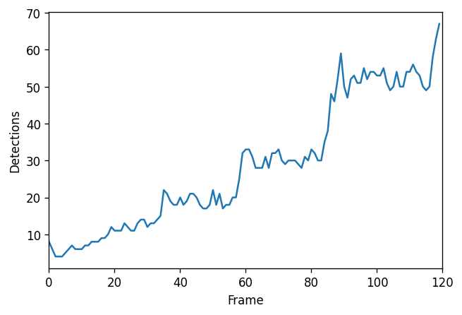
Based on these results, we can draw a plot of the number of detections as function of time:
import matplotlib.pyplot as plt

vc = df['frame'].value_counts()  # Count the number of detections per frame

fig, ax = plt.subplots(figsize=(6, 4), dpi=120)
ax.plot([vc[k] for k in range(len(image))])
ax.set_xlim(0, len(image))
ax.set_xlabel('Frame')
ax.set_ylabel('Detections')
plt.show()
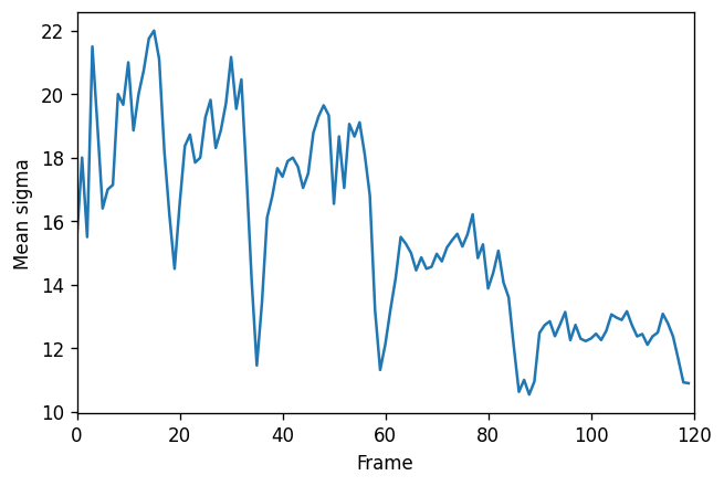
We can also plot the mean value of sigma in every frame. It looks like there is a pattern!
mean_sigmas = df.groupby('frame').mean()['sigma'].values

fig, ax = plt.subplots(figsize=(6, 4), dpi=120)
ax.plot(mean_sigmas)
ax.set_xlim(0, len(image))
ax.set_xlabel('Frame')
ax.set_ylabel('Mean sigma')
plt.show()
Particle tracking#
The next step in our analysis is to track individual cells over time. To do this, we need to compute a linkage between objects detected in consecutive frames. In Python, Trackpy is a package for particle tracking in 2D, 3D, and higher dimensions. We’ll use Trackpy’s link function, which implements the Crocker-Grier algorithm for calculating the linkage between objects.
# Compute the linkage using Trackpy.
linkage_df = tp.link(df, search_range=30, memory=3)

# This line is used to add the "length" column of the DataFrame.
linkage_df = linkage_df.merge(
    pd.DataFrame({'length': linkage_df['particle'].value_counts()}),
    left_on='particle', right_index=True
)

# The DataFrame now has a `particle` column identifying the particle ID and a `length` column corresponding to the track length.
linkage_df.head()
Frame 119: 67 trajectories present.
| y | x | sigma | frame | particle | length | |
|---|---|---|---|---|---|---|
| 0 | 268.0 | 560.0 | 24.0 | 0 | 0 | 5 |
| 1 | 148.0 | 384.0 | 24.0 | 0 | 1 | 2 |
| 2 | 364.0 | 380.0 | 24.0 | 0 | 2 | 37 |
| 3 | 248.0 | 188.0 | 24.0 | 0 | 3 | 7 |
| 4 | 116.0 | 332.0 | 6.0 | 0 | 4 | 3 |
Visualization in Napari#
The results of our tracking function can be visualized in Napari using the Tracks layer. The tracks data associated with it should be a 2D Numpy array of shape (N, 4) representing four columns: the track ID, frame ID, Y coordinate and X coordinate.
We can also add a separate Points layer to visualize the results of the spot detection.
# Extract data for the Napari viz
points = linkage_df[['frame', 'y', 'x']].values.astype(float)
sigmas = linkage_df['sigma'].values.astype(float)
lengths = linkage_df['length'].values.astype(float)
tracks = linkage_df[['particle', 'frame', 'y', 'x']].values.astype(float)

# Create the Napari Viewer setup. `view_image`` is a shortcut for `napari.Viewer().add_image()`.
viewer = napari.view_image(image)

# Visualize the results of the spot detection
viewer.add_points(
    points,
    name='Detections (LoG)',
    face_color='sigma',
    opacity=0.7,
    edge_width=0.0,
    size=sigmas+1,  # The size of the points can be parametrized
    features={'sigma': sigmas}  # Used to colorize the points
)

# Visualize the tracking results
viewer.add_tracks(
    tracks,
    name='Tracks (Trackpy)',
    tail_width=4,
    color_by='length',
    properties={'length': lengths}  # Colorize the tracks by length
)

# Take a screenshot
from napari.utils import nbscreenshot
nbscreenshot(viewer, canvas_only=True)
/home/wittwer/miniconda3/envs/image-analysis-field-guide/lib/python3.9/site-packages/napari/layers/tracks/tracks.py:620: UserWarning: Previous color_by key 'length' not present in features. Falling back to track_id
  warn(

Conclusion#
In this notebook, we have prototyped an image processing pipeline to detect and track cells in a timeseries. We have seen how the Tracks and Points layers of Napari can help us visualize the results of our analysis.
Going further#
Have a look at our collections of learning resources, jupyter notebooks, and softeware tools related to Tracking on our topic page.