n-D Image segmentation and visualization in Napari#
This notebook will give you a practical introduction to the Napari viewer.
Napari is a general-purpose N-dimensional image viewer based on Python. It is designed for browsing, annotating, and analyzing large multi-dimensional images. By integrating closely with Python, napari can be easily coupled to machine learning and image analysis libraries (e.g. scikit-image, scikit-learn, TensorFlow, PyTorch) enabling a user-friendly and automated analysis.
Setup#
First, make sure that you are executing this notebook in an environment with napari installed.
import napari
from napari.utils import nbscreenshot
Tip
If you are executing this notebook on a Jupyter Hub, launch a Remote Desktop from the start menu to be able to see the Napari Viewer in it.
Get the data#
The 3D image we’ll use in this tutorial is available for download on Zenodo (grains.tif).
In the cell below, we use a Python package called pooch to automatically download the image from Zenodo.
from shared_data import DATASET
image_file = DATASET.fetch("grains.tif")
image_file
'/home/wittwer/.cache/field-guide/grains.tif'
Read the image#
We’ll use the imread function from Scikit-image to read our TIF image.
from skimage.io import imread
image = imread(image_file)
print(f'Loaded image in an array of shape: {image.shape} and data type {image.dtype}')
print(f'Intensity range: [{image.min()} - {image.max()}]')
Loaded image in an array of shape: (400, 250, 250) and data type uint16
Intensity range: [0 - 65535]
n-D Image Visualization in Napari#
Napari is an open source Python-based viewer that supports full 3D rendering and visualization of large n-dimensional images. Communication between the viewer and the jupyter notebook is bidirectionnal. You can interactively load data from the Jupyter notebook into the viewer and control all of the viewer’s features programmatically.
1. Launching the Napari viewer#
You can run the code below to open the Napari viewer.
viewer = napari.Viewer();
Napari should have appeared in a seperate window. This is normal! You should keep the Napari viewer open while you run the next cells of this notebook.
Note
Unlike other jupyter widgets, napari is not embedded inside the jupyter notebook. This is because the graphical parts of napari are written in Qt, making it hard to embed on the web.
Tip
Use the shortcut Alt + Tab to rapidly switch between the Napari viewer and your Jupyter notebook window.
2. Adding an image#
You can load image data into the viewer either by drag-and-dropping image files directly onto it, or by programmatically calling add_image() from the notebook. The code below will load our image into the viewer.
viewer.add_image(image)
nbscreenshot(viewer)

You can check that the image is now opened in the viewer. For navigation, use the following commands:
Navigation |
Command |
|---|---|
Rotate (in 3D view) |
Left click & drag |
Pan (in 3D view) |
|
Zoom |
Right click & drag or mouse wheel |
Scroll slices (in 2D view) |
|
Toggle 2D/3D view |
|
Toggle grid view |
|
Toggle layer visibility |
|
You can access the layers list and the data in each layer through viewer.layers. When you change a property of a layer, such as the data it contains or its rendering parameters, the viewer will immediately update.
Tip
You can adjust a layer’s opacity to see the change how much you see of the layers that are “under” it.
For example, to adjust the contrast limits of an image layer:
viewer.layers['image'].contrast_limits
[0.0, 64871.0]
viewer.layers['image'].contrast_limits = (10_000, 60_000)
viewer.layers['image'].colormap = 'magma'
viewer.layers['image'].rendering = 'attenuated_mip'
You can check that the image rendering has changed in the viewer according to what you specified.
3. Image processing#
If you use Python to address your image analysis problem, you will likely have to apply multiple operations to your images successively. Napari can let you visualize the intermediate results of your image processing interactively.
For example, let’s segment individual grains in the image. First, we use Otsu’s method to produce a binary mask separating the foreground from the background. We then add the foreground as a Labels layer in Napari.
Napari supports seven different layer types, each corresponding to a different data type, visualization, and interactivity. Learn more about the available layer types in the official documentation.

viewer.layers['image'].colormap = 'gray' # reset the colormap of the image to gray
from skimage.filters import threshold_otsu
foreground = image >= threshold_otsu(image)
viewer.add_labels(foreground)
nbscreenshot(viewer)

You can toggle the grid mode (overlay versus side-by-side view of the layers) by holding Ctrl + G or (as with everything else) you can set this property from the notebook.
viewer.grid.enabled = True
def screenshot_view(viewer, canvas_only=False):
"""A custom screenshot view of the Napari viewer."""
viewer.dims.ndisplay = 3 # Activate 3D view
viewer.reset_view()
viewer.camera.angles = [0, 10, 80]
return nbscreenshot(viewer, canvas_only=canvas_only)
# Take a screenshot of the Viewer
screenshot_view(viewer)

Next, we compute the Euclidean distance transform of our binary image, which gives an estimate, for each pixel, of the distance to the closest boundary. Once again, we can use Napari to visualize the result.
from scipy.ndimage import distance_transform_edt
distance_img = distance_transform_edt(foreground)
viewer.add_image(distance_img, name='distance', colormap='viridis', opacity=0.5)
# Take a screenshot
screenshot_view(viewer, canvas_only=True)

Then, we detect local maxima in the distance image to use them as seed points. In napari, we can display the maxima in a layer of type Points.
import numpy as np
from skimage.feature import peak_local_max
from skimage.morphology import label
peaks = peak_local_max(distance_img, labels=label(foreground), min_distance=5)
viewer.add_points(peaks, name='peaks', size=4, face_color='red', opacity=0.7);
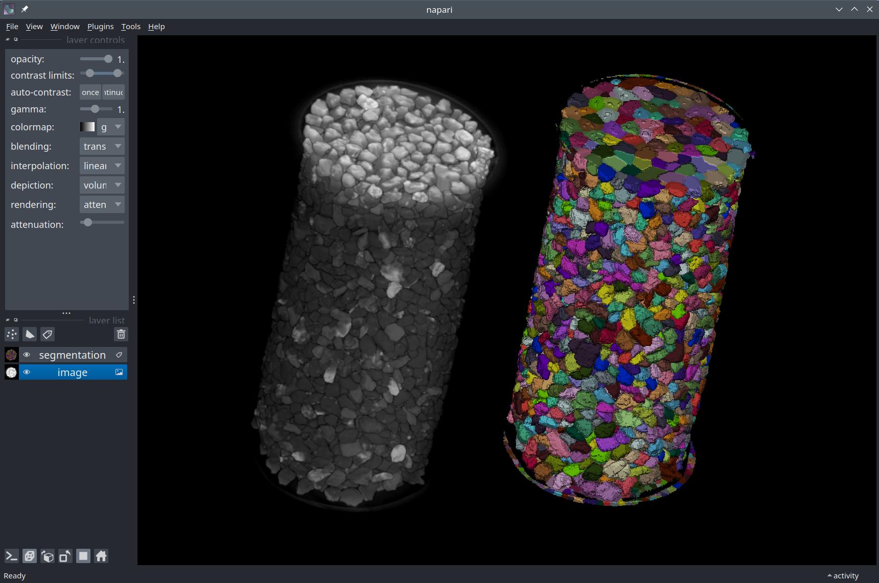
Finally, we compute a watershed segmentation of the grains using the detected peaks and we show the result in a Labels layer in Napari.
from skimage.segmentation import watershed
def peaks_to_markers(peaks):
"""Returns watershed markers from peaks data."""
peaks_x, peaks_y, peaks_z = peaks.astype('int').T
seeds = np.zeros(image.shape, dtype=bool)
seeds[(peaks_x, peaks_y, peaks_z)] = 1
# Label the marker points
markers = label(seeds)
return markers
# We do some minor tweaking to get the peaks data into the right format for watereshed
markers = peaks_to_markers(peaks)
# Watershed segmentation
particle_labels = watershed(-distance_img, markers, mask=foreground)
# Display the segmentation in a `Labels` layer
viewer.add_labels(particle_labels, name='segmentation')
# Take a screenshot
screenshot_view(viewer, canvas_only=True)

You could spend time perfecting this segmentation by adding more operations (e.g. denoising, background subtraction…) or optimizing algorithmic parameters. The important thing to remember is that with Napari, you can always visualize intermediate stages of image processing, giving you full control over your workflow.
You can also use Napari to interactively edit data in the layers (for example to correct segmentation results). You can add or remove points, or shapes, to create annotations. If you are interested in using Napari as an annotation tool, have a look at an example here.
4. Plugins#
Napari offers a range of community-developed plugins to extend the capabilities of the viewer. You can browse existing plugins on the Napari Hub.
An example of Plugin is napari-skimage-regionprops, which lets you measure the properties of objects. To install this plugin, open the “Plugins” menu from within the napari application, select “Install/Uninstall Package(s)…” and look for the plugin in the list. Alternatively, you can install the pluging using pip install napari-skimage-regionprops from your terminal.
With the plugin installed, you can run the cell below to add a parametric image in which the grains are color-coded based on their size.
# To run this cell, you should first install the plugin napari-skimage-regionprops from the Plugins menu in Napari
from skimage.measure import regionprops_table
from napari_skimage_regionprops import visualize_measurement_on_labels
# Compute region properties
statistics = regionprops_table(particle_labels, properties=['area'])
# Add the statistics as properties of the layer
label_image = viewer.layers['segmentation']
label_image.properties = statistics
# Compute the parametric image
parametric_image = visualize_measurement_on_labels(label_image, 'area')
# Display it
viewer.add_image(parametric_image, name="volume", colormap='jet')
# Take a screenshot
screenshot_view(viewer, canvas_only=True)
/tmp/ipykernel_38638/3299990140.py:13: DeprecationWarning: Call to deprecated function (or staticmethod) visualize_measurement_on_labels. (visualize_measurement_on_labels() is deprecated. Use map_measurements_on_labels() instead)
parametric_image = visualize_measurement_on_labels(label_image, 'area')

Conclusion#
We’ve now seen how to use Napari to visualize a 3D image, including looking at 2D slices and a 3D rendering. We’ve also seen that properties of the image viewer and of the loaded layers can be controlled both from the GUI interface and from the Jupyter notebook. Using Napari and Jupyter interactively, we were able to visualize intermediate steps of an image processing pipeline for segmentation, taking advantage of the different layer types available.