📐 Introduction to image registration#
In this notebook, we will use Python to automatically align a pair of 3D images onto one another using digital image correlation (DIC).
DIC is commonly used for image registration and for stabilizing a sequence of images by compensating camera movement, for tracking the movement and deformation of objects, and for image stitching of multiple fields of view, for example.
Tip
To learn more about DIC and spam, have a look at these resources:
Setup#
Check that you have all the necessary packages installed, including napari and spam.
import napari
from napari.utils import nbscreenshot
import spam.DIC
import spam.deformation
Tip
If you are executing this notebook on a Jupyter Hub, launch a Remote Desktop from the start menu to be able to see the Napari Viewer in it.
Get the data#
The image we’ll use in this tutorial is available for download on Zenodo (snow_3d.tif). The data represents snow grains which were CT scanned at 15 μm/px. It comes from an experiment by Peinke et al. from CEN / CNRM / Météo-France - CNRS. The sample was scanned in the Laboratoire 3SR micro-tomograph.
In the cell below, we use a Python package called pooch to automatically download the image from Zenodo.
from shared_data import DATASET

image_file = DATASET.fetch('snow_3d.tif')

image_file
'/home/wittwer/.cache/field-guide/snow_3d.tif'
Read the image#
We use the imread function from Scikit-image to read our TIF image.
from skimage.io import imread

image = imread(image_file)

print(f'Loaded image in an array of shape: {image.shape} and data type {image.dtype}')
print(f'Intensity range: [{image.min()} - {image.max()}]')
Loaded image in an array of shape: (100, 100, 100) and data type uint16
Intensity range: [6237 - 40103]
Load the image into Napari#
Let’s open a viewer and load our image to have a look at it.
viewer = napari.Viewer(title="Image registration")
viewer.grid.enabled = True
viewer.add_image(image, colormap='magenta', name='Fixed image')

# Take a screenshot
viewer.reset_view()
nbscreenshot(viewer, canvas_only=True)

Generate a misaligned image#
For the sake of this demonstration, we will rotate and translate the original image by an arbitrary amount to produce a misaligned image. We will then attempt to register this misaligned image back onto the orginal image. In this way, since we know the true transformation, we will be able to compare it to the transformation determined by the DIC algorithm.
In reality, the fixed and moving images would be acquired independently - but the concept is the same!
# Choose a transformation to apply to the original image
transformation = {
    't': [0.0, 3.0, 2.5],  # Translation in Z, Y, X
    'r': [3.0, 0.0, 0.0],  # Rotation (in degrees) around Z, Y, X
}

# The 4 x 4 matrix `Phi` represents the 3D transformation applied to the image.
# Learn more: https://ttk.gricad-pages.univ-grenoble-alpes.fr/spam/tutorials/tutorial-02a-DIC-theory.html
Phi_ground_truth = spam.deformation.computePhi(transformation)

Phi_ground_truth
array([[ 1.   ,  0.   ,  0.   ,  0.   ],
       [ 0.   ,  0.999, -0.052,  3.   ],
       [ 0.   ,  0.052,  0.999,  2.5  ],
       [ 0.   ,  0.   ,  0.   ,  1.   ]])
We generate our moving image by applying the transform:
# The moving image is rotated and translated with respect to the original image
moving_image = spam.DIC.applyPhi(image, Phi=Phi_ground_truth)

viewer.add_image(moving_image, colormap='blue', name="Moving image")

viewer.reset_view()
nbscreenshot(viewer, canvas_only=True)

Registration by the optical flow method#
Now that we have a moving_image, we can try to align it onto the original image using DIC.
We use the register function from spam to do that. The function returns a dictionary containing information about the registration (convergence, error…), including an estimate of the Phi deformation matrix that brings the moving image onto the original image.
reg = spam.DIC.register(moving_image, image)

Phi = reg.get('Phi')
error = reg.get('deltaPhiNorm')

transformation_estimate = spam.deformation.decomposePhi(Phi)

print(f"Translation (ZYX): {transformation_estimate['t']}")
print(f"Rotation (deg) (ZYX): {transformation_estimate['r']}")
Translation (ZYX): [ 0.    -3.127 -2.34 ]
Rotation (deg) (ZYX): [-3.  0. -0.]
This result is almost the exact opposite of the transform we applied to the original image, so it looks like the registration was successful!
Apply the transform#
Let’s apply our esimated transformation to the moving image to check that this transformation brings it back onto the original image.
registered = spam.DIC.applyPhi(moving_image, Phi=Phi)

# Trick: the `additive` blending mode applied to a layer with colormap `cyan` overlayed on a layer with
# colormap `magenta` leads to a white color where the intensity in both layers is the same.
viewer.add_image(registered, name="Registered", colormap='cyan', blending='additive')

# In Napari, you can display some text in the top-left part of the window, for example:
viewer.text_overlay.visible = True
viewer.text_overlay.text = f'deltaPhiNorm = {error:.2e}'

viewer.reset_view()
nbscreenshot(viewer, canvas_only=True)

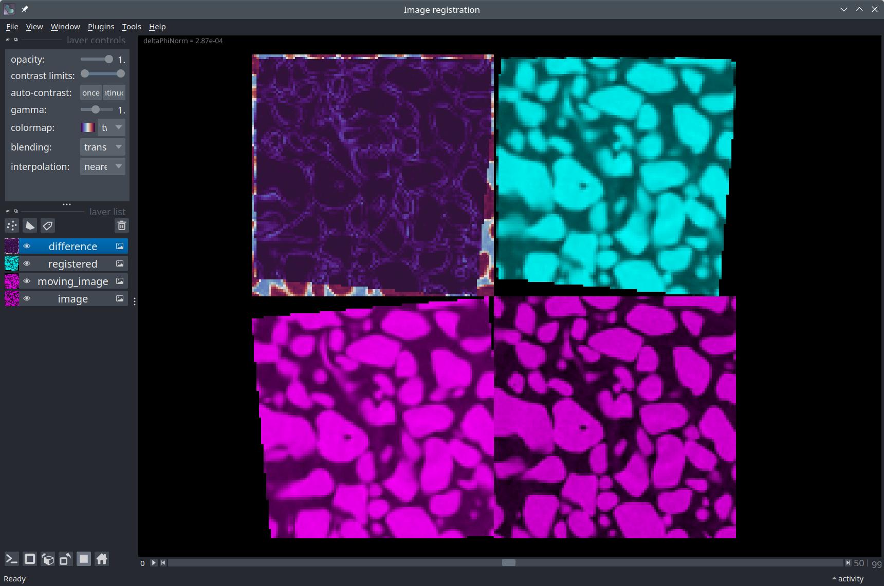
Compute the error pixel-wise#
Finally, we can compute the pixel-wise squared difference between the registered and original image to visualize the error.
import numpy as np

difference = np.square(registered - image)

viewer.add_image(difference, name="Squared difference", colormap='twilight_shifted')

viewer.reset_view()
nbscreenshot(viewer, canvas_only=True)

Displacement vectors#
Finally, for the sake of visualization, we generate a grid of points onto our 3D image and show how they get displaced by the registration transform.
node_spacing = (10, 10, 10)  # The pixel spacing between each vector in the grid, in Z/Y/X.

node_positions = spam.DIC.makeGrid(image.shape, node_spacing)[0]

# We apply our transform to each point in the grid to displace it.
# Add a `1` to each node position to express it in homogeneous coordinates
node_positions = np.hstack((node_positions, np.ones(len(node_positions))[None].T))

# Displace the nodes (around the center of the image - not the corner)
origin_point = np.array(image.shape) // 2
origin_point = np.hstack((origin_point, [0.0])).astype(float)
displaced_nodes = np.vectorize(lambda node: np.matmul(Phi, node - origin_point) + origin_point, signature='(n)->(n)')(node_positions)

# Homogeneous -> Cartesian
displaced_nodes = displaced_nodes[:, :-1]
node_positions = node_positions[:, :-1]

# Get the vectors in shape (N, 2, 3)
displacements = displaced_nodes - node_positions
displacement_vectors = np.concatenate((node_positions[np.newaxis], displacements[np.newaxis]))
displacement_vectors = np.swapaxes(displacement_vectors, 0, 1)

# Visualize the vectors
viewer.add_vectors(displacement_vectors, name='Displacement', edge_width=0.7, opacity=1.0, ndim=3)

viewer.reset_view()
nbscreenshot(viewer, canvas_only=True)

Conclusion#
In this notebook, we have had a first look at digital image correlation in Python using the spam package. We used Napari to visualize the results of the registration.
Going further#
Have a look at our collections of learning resources, jupyter notebooks, and softeware tools related to Image registration on our topic page.