✂️ Introduction to image segmentation

This tutorial will give you a practical introduction to image segmentation. We’ll aim to produce a segmentation mask that identifies objects of interest in an image. We will attempt to separate the objects from the background. Then, we’ll see how to distinguish individual objects. Finally, we’ll show how to measure properties (size, shape) of these objects.

Setup

First, make sure that you are executing this notebook in an environment with all the necessary packages installed. We’ll import every function and library that we need in the cell below. We’ll use these imports progressively in the notebook.

import ipywidgets
import numpy as np
import pandas as pd
import scipy.ndimage as ndi
import matplotlib.pyplot as plt
import skimage.data
from skimage.io import imshow
from skimage.exposure import histogram
from skimage.filters import sobel, threshold_otsu
from skimage.measure import regionprops_table
from skimage.segmentation import watershed
from skimage.color import label2rgb

Load an image

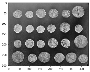
We will use the coins image from skimage.data as an example. This image shows several coins outlined against a darker background.

image = skimage.data.coins()

print(f'Loaded image in an array of shape: {image.shape} and data type {image.dtype}')
print(f'Intensity range: [{image.min()} - {image.max()}]')

Loaded image in an array of shape: (303, 384) and data type uint8
Intensity range: [1 - 252]

This is what our image looks like:

imshow(image)

<matplotlib.image.AxesImage at 0x71cd2545dfa0>

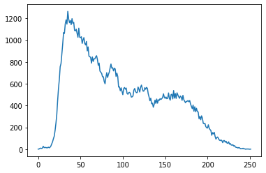
We can also plot the image histogram:

hist, hist_centers = histogram(image)

plt.plot(hist)
plt.show()

Thresholding

First, we are going to attempt to segment the image by thresholding the graylevel intensities. For this, we select a threshold, and then apply it to the image. All the pixel intensity values above the selected threshold become 1, and the rest 0. This type of image array is known as a binary mask.

To create a suitable binary mask, the challenge is to find a threshold value that works well for our image (if that is possible), that is, which accurately separates the foreground from the background pixels.

In the cell below, we show you a way of creating an interactive threshold function using ipywidgets. Move the slider to see the effect on the segmentation mask.

def segment_image(threshold):
    binary_image = image > threshold
    fig, ax = plt.subplots(1, 2, figsize=(12, 6))
    ax[0].imshow(image, cmap='gray')
    ax[0].set_title('Original Image')
    ax[0].axis('off')
    ax[1].imshow(binary_image, cmap='gray')
    ax[1].set_title('Segmented Image')
    ax[1].axis('off')
    plt.show()

threshold_slider = ipywidgets.IntSlider(
    value=threshold_otsu(image),
    min=0,
    max=255,
    step=1,
    description='Threshold:',
    continuous_update=True
)

ipywidgets.interactive(segment_image, threshold=threshold_slider)

Automatic thresholding

There are methods to automatically select intensity thresholds based on the image histogram. One of these methods is Otsu thresholding. You can try the following:

from skimage.filters import threshold_otsu
threshold = threshold_otsu(blobs)
binary_blobs = blobs < threshold

However, this only selects a good guess for a threshold.

It looks like simply thresholding the image leads either to missing significant parts of the coins, or to merging parts of the background with the coins. This is due to the inhomogeneous lighting of the image.

Therefore, we’ll try a more advanced segmentation approach.

Watershed segmentation

The watershed transform floods an image of elevation starting from markers, in order to determine the catchment basins of these markers. Watershed lines separate these catchment basins, and correspond to the desired segmentation.

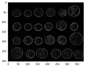
The choice of the elevation map is critical for good segmentation. Here, we use the Sobel operator for computing the amplitude of the intensity gradient in the original image (the edges):

edges = sobel(image)

imshow(edges)

<matplotlib.image.AxesImage at 0x71cd242fa3a0>

Let us first determine markers of the coins and the background. These markers are pixels that we can label unambiguously as either object or background. Here, the markers are found at the two extreme parts of the histogram of gray values:

markers = np.zeros_like(image)
markers[image < 30] = 1
markers[image > 150] = 2

Let us now compute the watershed transform:

segmentation = watershed(edges, markers)

imshow(segmentation)

/home/wittwer/miniconda3/envs/image-analysis-field-guide/lib/python3.9/site-packages/skimage/io/_plugins/matplotlib_plugin.py:149: UserWarning: Low image data range; displaying image with stretched contrast.
  lo, hi, cmap = _get_display_range(image)

<matplotlib.image.AxesImage at 0x71cd2423bfd0>

With this method, the result is satisfying for all coins. Even if the markers for the background were not well distributed, the barriers in the elevation map were high enough for these markers to flood the entire background.

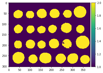
To further improve the segmentation, we remove a few small holes using the scipy.ndimage.binary_fill_holes() function:

segmentation = ndi.binary_fill_holes(segmentation - 1)

imshow(segmentation)

<matplotlib.image.AxesImage at 0x71cd241342e0>

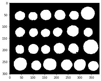
Our binary mask looks good. The next step is to distinguis the coins from each other, which we can do using an algorithm known as connected components labeling.

Connected component labeling

Conceptionally, label images are an extension of binary masks. In a label image, all pixels with value 0 correspond to background. Pixels with a value larger than 0 denote that the pixel belongs to an object and identifies that object with the given number. A pixel with value 1 belongs to first object and pixels with value 2 belongs to a second object and so on. When objects are labeled subsequently, the maximum value in a label mask corresponds to the number of objects in the image.

Let’s label all the coins in our binary mask using the ndi.label function from Scipy:

labeled_segmentation, _ = ndi.label(segmentation)

imshow(labeled_segmentation)

<matplotlib.image.AxesImage at 0x71cd240aea00>

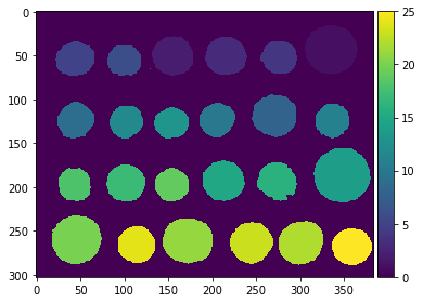
This is nice. Now, what if we want to measure some properties of our labeled objects, such as their size?

Measuring region properties

After segmenting and labeling objects in an image, we can measure properties of these objects. To read out properties from regions, we use the regionprops_table function from Scikit-image. We read the properties into a Pandas DataFrame, which is a common asset for data scientists.

properties = regionprops_table(labeled_segmentation, intensity_image=image, properties=['label', 'area', 'centroid', 'bbox', 'eccentricity', 'intensity_mean'])

df = pd.DataFrame(properties)

df.head()

	label	area	centroid-0	centroid-1	bbox-0	bbox-1	bbox-2	bbox-3	eccentricity	intensity_mean
0	1	2604.0	43.536866	334.656682	16	305	72	365	0.332340	156.808372
1	2	1653.0	50.774955	155.258923	28	132	74	179	0.294055	169.370841
2	3	1622.0	51.098644	215.235512	30	192	73	240	0.383282	157.607275
3	4	1225.0	52.389388	276.126531	34	255	72	297	0.388527	154.203265
4	5	1355.0	54.390406	44.177122	35	22	74	67	0.510381	167.821402

From there, we can study individual measurements or compute statistics on the whole dataset of detected objects. For example:

df.describe()

	label	area	centroid-0	centroid-1	bbox-0	bbox-1	bbox-2	bbox-3	eccentricity	intensity_mean
count	25.000000	25.000000	25.000000	25.000000	25.000000	25.000000	25.000000	25.000000	25.000000	25.000000
mean	13.000000	1557.800000	154.499355	189.403899	133.880000	167.600000	176.200000	212.120000	0.369585	162.924813
std	7.359801	625.452303	81.205187	102.941702	79.477104	101.027224	83.442595	104.973139	0.155395	16.668389
min	1.000000	2.000000	43.536866	43.690391	16.000000	18.000000	66.000000	63.000000	0.203215	130.988511
25%	7.000000	1175.000000	65.000000	102.291629	65.000000	84.000000	74.000000	124.000000	0.263170	153.616162
50%	13.000000	1471.000000	127.212628	172.303404	110.000000	144.000000	145.000000	201.000000	0.341121	159.189983
75%	19.000000	1765.000000	197.743056	273.524733	179.000000	251.000000	218.000000	297.000000	0.419496	171.959471
max	25.000000	3141.000000	267.864646	358.171044	248.000000	336.000000	289.000000	382.000000	1.000000	194.683380

To save the dataframe to disk conveniently, you could run dataframe.to_csv("blobs_analysis.csv").

Displaying a figure

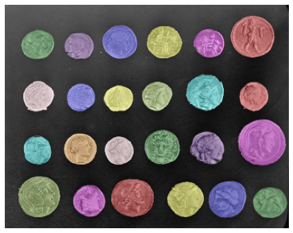
We use the label2rgb function from Scikit-image to display the segmentation overlaid on the original image.

fig, ax = plt.subplots(figsize=(12, 6))
rgb_composite = label2rgb(labeled_segmentation, image=image, bg_label=0)
ax.imshow(rgb_composite)
plt.axis('off')
plt.show()