🪄 Simple image denoising#
In this notebook, we will introduce image denoising in Python using Scikit-image.
If you haven’t already, we recommend you take a look at these tutorials before this one:
Introduction#
Image denoising is used to generate images with high visual quality, in which structures are easily distinguishable, and noisy pixels are removed. Denoised images are often more amendable to thresholding for segmentation.
To begin our image denoising demonstration, we will first import a few libraries:
Matplotlib to display images.
Numpy to manipulate numerical arrays.
import matplotlib.pyplot as plt
import numpy as np
We will also need scikit-image, which will provides us with image processing filters, algorithms, and utility functions (e.g. for loading images).
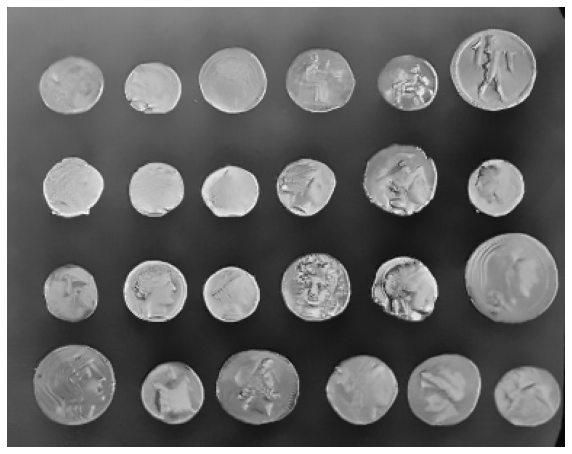
Let’s load the coins image from Scikit-image’s data module to use it as an example.
from skimage.data import coins

image = coins() # An example image

print(f"Image shape (px): {image.shape}. Min value = {image.min()}, Max value = {image.max()}. Data type: {image.dtype}")
Image shape (px): (303, 384). Min value = 1, Max value = 252. Data type: uint8
Let’s define a function that we can reuse to display images.
def display_image(image, title=''):
    fig, ax = plt.subplots(figsize=(10, 10))
    ax.imshow(image, vmin=0, vmax=255, cmap=plt.cm.gray)
    ax.set_title(title)
    ax.axis('off')
    plt.show()

    return fig

display_image(image)

Note
To read an image saved locally, you could use Scikit-image’s io (input-output) module and provide a path to your image file. For example:
from skimage import io

image = io.imread('/path/to/my_image.tif')

display_image(image)
Adding artificial noise to the image#
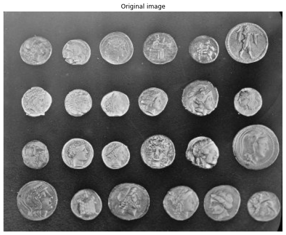
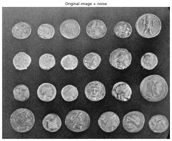
For the sake of this tutorial, we will add some Gaussian noise to our image to simulate a noisy acquisition.
noise = np.random.normal(loc=0, scale=10, size=image.shape)
noisy_image = image + noise
noisy_image = np.clip(noisy_image, 0, 255)

display_image(image, 'Original image')
display_image(noisy_image, 'Original image + noise')
Denoising techniques#
Let’s try denoising our image. To do this, we’ll first test the application of a gaussian filter and a median filter to the noisy image.
from skimage.filters import gaussian, median
The sigma parameter of the Gaussian filter controls the degree of blurring in the image. There is a trade-off between the intensity of the blurring and the preservation of fine details in the image.
Tip
Try applying different values of sigma and observe how it affects the resulting image!
denoised_image_gaussian = gaussian(noisy_image, sigma=1)

display_image(denoised_image_gaussian)
Let’s compare this method with the application of a median filter.
denoised_image_median = median(noisy_image)

display_image(denoised_image_median)

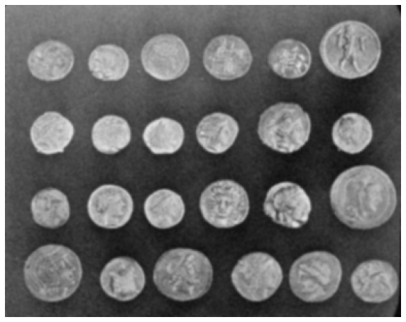
Finally, let’s use non-local means denoising. In this case, we also estimate the standard deviation of the noise from the image.
from skimage.restoration import denoise_nl_means, estimate_sigma
sigma_est = estimate_sigma(noisy_image)

print(f"Estimated standard deviation of the noise: {sigma_est:.1f}")
Estimated standard deviation of the noise: 11.6
Our estimate is not too far from the value of 10 that we have used when simulating the noise!
denoised_image_nl_means = denoise_nl_means(noisy_image, h=1.15*sigma_est, fast_mode=True, patch_size=5, patch_distance=6)

fig = display_image(denoised_image_nl_means)
As usual, to learn more about the functions we use, it’s a good idea to read their documentation.
help(denoise_nl_means)
Show code cell output
Help on function denoise_nl_means in module skimage.restoration.non_local_means:

denoise_nl_means(image, patch_size=7, patch_distance=11, h=0.1, fast_mode=True, sigma=0.0, *, preserve_range=False, channel_axis=None)
    Perform non-local means denoising on 2D-4D grayscale or RGB images.

    Parameters
    ----------
    image : 2D or 3D ndarray
        Input image to be denoised, which can be 2D or 3D, and grayscale
        or RGB (for 2D images only, see ``channel_axis`` parameter). There can
        be any number of channels (does not strictly have to be RGB).
    patch_size : int, optional
        Size of patches used for denoising.
    patch_distance : int, optional
        Maximal distance in pixels where to search patches used for denoising.
    h : float, optional
        Cut-off distance (in gray levels). The higher h, the more permissive
        one is in accepting patches. A higher h results in a smoother image,
        at the expense of blurring features. For a Gaussian noise of standard
        deviation sigma, a rule of thumb is to choose the value of h to be
        sigma of slightly less.
    fast_mode : bool, optional
        If True (default value), a fast version of the non-local means
        algorithm is used. If False, the original version of non-local means is
        used. See the Notes section for more details about the algorithms.
    sigma : float, optional
        The standard deviation of the (Gaussian) noise.  If provided, a more
        robust computation of patch weights is computed that takes the expected
        noise variance into account (see Notes below).
    preserve_range : bool, optional
        Whether to keep the original range of values. Otherwise, the input
        image is converted according to the conventions of `img_as_float`.
        Also see https://scikit-image.org/docs/dev/user_guide/data_types.html
    channel_axis : int or None, optional
        If None, the image is assumed to be a grayscale (single channel) image.
        Otherwise, this parameter indicates which axis of the array corresponds
        to channels.

        .. versionadded:: 0.19
           ``channel_axis`` was added in 0.19.

    Returns
    -------
    result : ndarray
        Denoised image, of same shape as `image`.

    Notes
    -----

    The non-local means algorithm is well suited for denoising images with
    specific textures. The principle of the algorithm is to average the value
    of a given pixel with values of other pixels in a limited neighborhood,
    provided that the *patches* centered on the other pixels are similar enough
    to the patch centered on the pixel of interest.

    In the original version of the algorithm [1]_, corresponding to
    ``fast=False``, the computational complexity is::

        image.size * patch_size ** image.ndim * patch_distance ** image.ndim

    Hence, changing the size of patches or their maximal distance has a
    strong effect on computing times, especially for 3-D images.

    However, the default behavior corresponds to ``fast_mode=True``, for which
    another version of non-local means [2]_ is used, corresponding to a
    complexity of::

        image.size * patch_distance ** image.ndim

    The computing time depends only weakly on the patch size, thanks to
    the computation of the integral of patches distances for a given
    shift, that reduces the number of operations [1]_. Therefore, this
    algorithm executes faster than the classic algorithm
    (``fast_mode=False``), at the expense of using twice as much memory.
    This implementation has been proven to be more efficient compared to
    other alternatives, see e.g. [3]_.

    Compared to the classic algorithm, all pixels of a patch contribute
    to the distance to another patch with the same weight, no matter
    their distance to the center of the patch. This coarser computation
    of the distance can result in a slightly poorer denoising
    performance. Moreover, for small images (images with a linear size
    that is only a few times the patch size), the classic algorithm can
    be faster due to boundary effects.

    The image is padded using the `reflect` mode of `skimage.util.pad`
    before denoising.

    If the noise standard deviation, `sigma`, is provided a more robust
    computation of patch weights is used.  Subtracting the known noise variance
    from the computed patch distances improves the estimates of patch
    similarity, giving a moderate improvement to denoising performance [4]_.
    It was also mentioned as an option for the fast variant of the algorithm in
    [3]_.

    When `sigma` is provided, a smaller `h` should typically be used to
    avoid oversmoothing.  The optimal value for `h` depends on the image
    content and noise level, but a reasonable starting point is
    ``h = 0.8 * sigma`` when `fast_mode` is `True`, or ``h = 0.6 * sigma`` when
    `fast_mode` is `False`.

    References
    ----------
    .. [1] A. Buades, B. Coll, & J-M. Morel. A non-local algorithm for image
           denoising. In CVPR 2005, Vol. 2, pp. 60-65, IEEE.
           :DOI:`10.1109/CVPR.2005.38`

    .. [2] J. Darbon, A. Cunha, T.F. Chan, S. Osher, and G.J. Jensen, Fast
           nonlocal filtering applied to electron cryomicroscopy, in 5th IEEE
           International Symposium on Biomedical Imaging: From Nano to Macro,
           2008, pp. 1331-1334.
           :DOI:`10.1109/ISBI.2008.4541250`

    .. [3] Jacques Froment. Parameter-Free Fast Pixelwise Non-Local Means
           Denoising. Image Processing On Line, 2014, vol. 4, pp. 300-326.
           :DOI:`10.5201/ipol.2014.120`

    .. [4] A. Buades, B. Coll, & J-M. Morel. Non-Local Means Denoising.
           Image Processing On Line, 2011, vol. 1, pp. 208-212.
           :DOI:`10.5201/ipol.2011.bcm_nlm`

    Examples
    --------
    >>> a = np.zeros((40, 40))
    >>> a[10:-10, 10:-10] = 1.
    >>> rng = np.random.default_rng()
    >>> a += 0.3 * rng.standard_normal(a.shape)
    >>> denoised_a = denoise_nl_means(a, 7, 5, 0.1)
Conclusion#
In this tutorial, we have looked at three simple methods for denoising an image:
Applying a Gaussian filter
Applying a Median filter
Non-local means filtering
Going further#
There are many other powerful denoising techniques and algorithms, and much more to know. We recommend that you have a look at Scikit-image’s excellent resources on the topic.
You can also have a look at our collections of learning resources, jupyter notebooks, and software tools related to Image denoising on our topic page.